
Deducing Protein Sequence from Structure using a Graph Neural Network
A quick dive into the inverse protein folding model, ProteinMPNN

The Inverse Folding Problem
Why We Need Protein Sequences In Protein Design?
So far in this blog we’ve covered protein structure prediction, where we predict a protein’s structure given its amino acid sequence. Moreover, we’ve touched on protein structure generation, where we can generate brand new protein structures conditioned on some functional or structural criteria. But once we have “designed” our protein structure to bind to another protein or catalyze a reaction, how do we actually synthesize it, so we can test and use it? Unfortunately, just having the structure is not sufficient for synthesizing the protein. In fact, knowing the amino acid sequence of your protein is required! Why? Because of recombinant protein expression, the process for making proteins in vitro. Recombinant protein expression involves inserting a specific gene (piece of DNA) into bacteria to coax it into producing your protein. Remember, genes are templates used to create RNA (transcription), which in turn contain the recipe to construct proteins (translation). Because the mapping of gene sequences to RNA sequences and then to amino acid sequences is known, we can easily work backward to determine the gene sequence of any desired protein sequence.
Why Structure to Sequence is Hard?
While determining DNA sequence from protein sequence is relatively straightforward, deducing a protein sequence from its structure, a process called inverse folding, is not so easy. It should be easy though right? To determine a protein residue sequence from a structure, you need to figure out a) how many residues are in the structure, b) what order they are in the sequence, and c) which of the 20 amino acids each one is. The output of structure generation models like RFDiffusion is usually an ordered list of coordinates for each residue’s backbone atoms, which already covers a and b. RFDiffusion and similar models, however, do not output residue side chain coordinates (only backbone coordinates). Side chains are not only the distinguishing part of each of the 20 amino acid residue types, but they are also what give each residue its unique properties, which affects how it folds. Without side chain information it isn’t very straightforward to determine residue identity. By looking at how the residues fold and bind to each other in the structure, however, it can theoretically be inferred! Indeed, using structural cues to figure out which residue backbones correspond to which amino acid residues is exactly what ProteinMPNN does! In this post, we’ll cover how ProteinMPNN, a deep graph neural network model, tackles this structure-to-sequence inference problem.
Graph-Structured Input
To design protein sequences, ProteinMPNN formulates the input 3D structure as a graph. So what’s a graph and how do you structure your input to be like one?
What’s a graph and how is it used here?
A graph, G, is defined as a set of nodes or vertices, V, that are connected to each other by edges, E. If every node is attached to every other node in the graph, then the graph is “fully connected”. Most graphs, however, are usually more sparsely connected. While graphs are a mathematical construct, they are very useful as a way to model relationships between entities in the real world. For example, graphs can model social networks, where each person’s LinkedIn profile is a node and if two people are “connected” (not a coincidence that LinkedIn uses this terminology!), then there is an edge between them. In the case of ProteinMPNN, graphs are used to model protein structure, where each node is a residue and each edge encodes the interaction between a pair of residues. If we remember from previous posts, AlphaFold2 and RFDiffusion will model the 3D coordinate data from PDB as local frames (which encode a local coordinate system for each residue) and pairwise distances and angles between residues or atoms in the residues. We can think of ProteinMPNN’s graph-structured input as just another way to pre-process the “raw” structure data from PDB.
Why graph-structured input?
As we know for structure prediction models, residues from different parts of a sequence can interact and bind to each other resulting in very complicated 3D folds. As such, structure prediction models, like AlphaFold, will model the interaction between every possible pair of residues in order to figure out which ones fold onto each other. In inverse folding, on the other hand, we know what the structure looks like, so we are more interested in using our knowledge of how residues interact in space to figure out which amino acids they are. Instead of capturing long-range dependencies we just want to look at short range local dependencies between residues that are close to each other. Graphs are perfect for capturing short range interactions because we will only represent edges between nodes (residues) that are nearby.
Capturing and processing local, sparse structure is also computationally cheaper. Encoding a representation to capture the interactions between a residue with every other residue, as AlphaFold does, has a computational time complexity of O(N^2). This means that as the number of residues increases by doubling, the computational cost (the time to compute the representation) is quadrupled and if the sequence length quadruples, the computational cost increases 16-fold! Basically, it doesn’t scale very nicely. With operations on graphs, where we’ll maybe only try to compute the interaction between a residue and k of its neighbors, the time complexity is O(Nk). This means the compute cost scales linearly with the number of residues: if we quadruple our protein sequence length, the time to compute our interactions similarly quadruples.
ProteinMPNN Inputs
Ok so how does ProteinMPNN specifically formulate the xyz-coordinates of PDB protein structure as a graph? To make a graph representation you just need a set of node representations for each residue and edge representations for pairs of residues.
ProteinMPNN computes an edge feature, E, for a given pair of residues by concatenating the distance between the two residues in 3D space with the relative positional encoding of the residue pair. The distance between two residues in 3D space is computed as distances between each of the backbone atoms (nitrogen, alpha carbon, carbonyl carbon, oxygen, and a virtual beta carbon1) in one residue with the corresponding backbone atom of the other residue. These distances are encoded using 16 radial basis functions, whereby 16 distances are chosen and we evaluate our interatomic distances under gaussians centered at each of these 16 distances to convert each scalar interatomic distance to a 16-dimensional vector. The relative positional encoding measures how far apart the residues are in the sequence (remember we know the order of the residues in the sequence, but not which amino acid each is) by counting how many residues away they are from each other. They bin this relative position into buckets between -32 and 32, where -32 and 32 represent 32 residues away and greater. In addition, for multi-chain proteins (protein structures that come from distinct sequences that then bind together after folding), there is a 33rd bin to denote that this pair of residues come from different chains.
The node features, V, are initialized to all zeros and iteratively updated as they processed by the model in the forward pass.
The ProteinMPNN Architecture
ProteinMPNN is an encoder-decoder architecture that falls uunder a family of graph neural networks called Message Passing Neural Networks (MPNN’s).
Message Passing Neural Networks (MPNN’s)
Message Passing Neural Networks (MPNN’s) are first described in this paper as a family of neural networks that operate on graph structured inputs (node features and edge features). In message passing neural networks: a “message” is computed between two neighboring nodes, V_i and V_j, by combining the two node features along with the features for the edge between the nodes, E_ij and passing them through a small neural network. The architecture of the neural network and how these three features are combined varies across different instantiations of MPNN’s. The sum of the messages between the ith node and each of its neighbors are then used to update the ith node. In some MPNN’s, each message between two nodes is used to update the edge representation for those two nodes. MPNN’s usually apply the message passing phase multiple times to iteratively update the nodes. Each time message passing is applied, an updated node will encode information about nodes further and further away from its closest neighbors.
The Encoder-Decoder Architecture
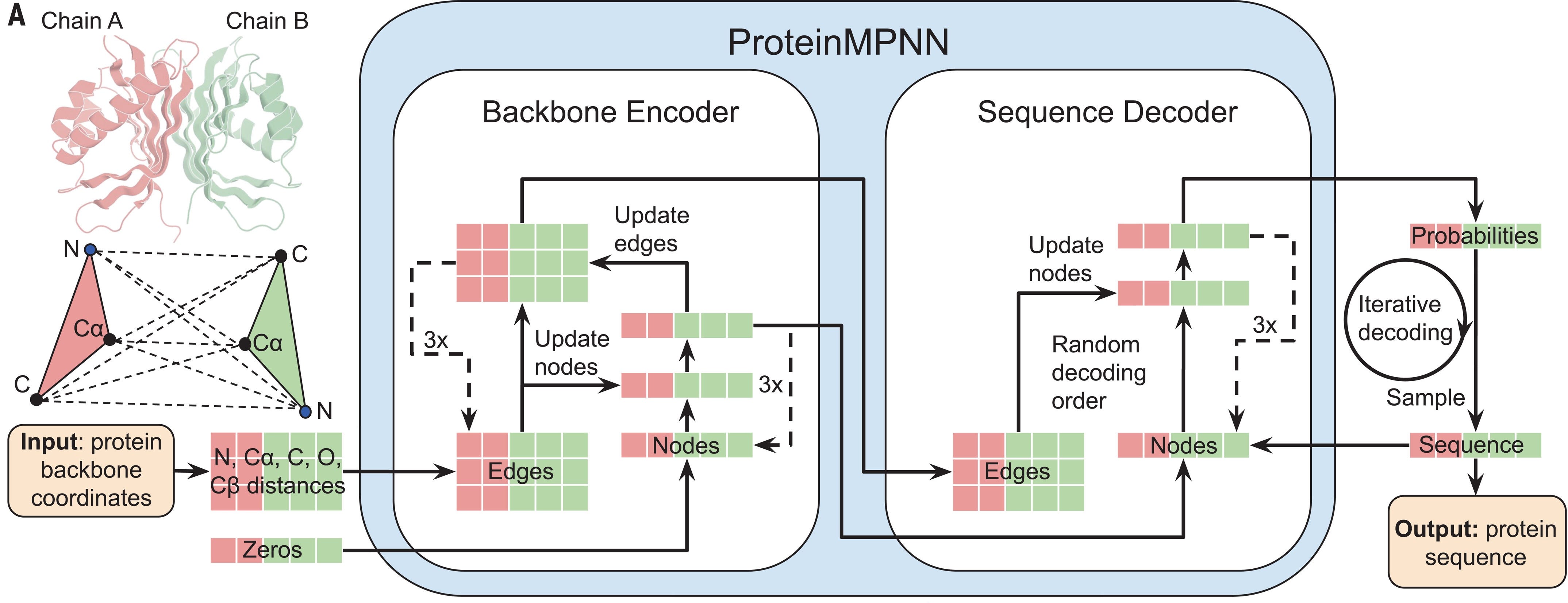
The ProteinMPNN architecture consists of a first an encoder, which uses message passing to iteratively refine the node and edge representations. The encoder is then followed by the decoder, which is a similar architecture to the encoder, but only updates the node representation. Then “decoded” node representation is processed by a linear classifier to predict its amino acid class.
The Encoder
To update a given node representation, V_i, the encoder first computes a “message”, M_ij, between it and one of its neighboring nodes, V_j by concatenating V_i, V_j, and E_ij, the edge between them. The message is computed by processing the concatenated vector with a 3-layer MLP with hidden dimension 128. The messages between V_i and its 30 closest neighbors (close as measured by the distance between V_i’s alpha carbon and the other nodes’ alpha carbons) are summed up to yield the node update, dV_i. Some further processing is then done to get the final update for V_i, which we will detail in the pseudocode. The edge representation, E_ij, is updated similarly by computing another “message”, M_ij, and processing that further. The encoder then repeats this process twice more before the node and edge representations are processed by the decoder. Here is some PyTorchy pseudocode (not actual code even though it looks like it!):
def encoder_layer(v, e, k=30):
    for i in range(v.shape[0]):
        vi_neighbor_inds = nearest_neighbors_ind(v[i], k)
        dvi = 0
        for j in vi_neighbor_inds:
            cat_ij = concat((v[i], v[j], e[i,j]))
            m_ij = MLP(layers=3, activation=gelu, hidden_dim=128)(cat_ij)
            dvi += m_ij
            de_ij = MLP(layers=3, activation=gelu, hidden_dim=128)(cat_ij)
            e[i,j] = LayerNorm(e[i,j] + dropout(de_ij))
        v[i] = LayerNorm(v[i] + dropout(dvi))
        dvi = MLP(layers=2, activation=gelu, hidden_dim=128)(v[i])
        v[i] = LayerNorm(v[i] + dropout(dvi))
    return v, e

def encoder(v, e):
    for _ in range(3):
        v, e = encoder_layer(v, e)
The Decoder
Unlike the encoder, the messages in the decoder are a function of the true protein sequence (amino acid residue labels) along with the node and edge representations. The catch is that the decoder messages are computed using a “causal” mask, which zeros out elements of the sequence that come after the residue the given node represents. For example, for updating node i, the ith and greater elements of the sequences are masked out, so that node i is decoded using only residues earlier in the sequence. This is done to enable “autoregressive” decoding at inference time. More on what that means in the inference section!
The decoder computes the node updates in almost exactly the same way as the encoder. The only difference is that for a given edge representation, E_ij, the jth element in the ground truth protein sequence, s[j], is concatenated to E_ij if i > j and otherwise, zeros are concatenated. After the decoder updates the node representation, each representation is mapped to a categorical probability distribution over amino acid classes using a linear layer plus softmax. Here is some PyTorchy pseudocode (not actual code even though it looks like it!):
def decoder_layer(v, e, s, i, k=30, output_s_pred=False):
        vi_neighbor_inds = nearest_neighbors_ind(v[i], k)
        dvi = 0
        for j in vi_neighbor_inds:
            mask_ij = (1 if i > j else 0)
            # concatenate sequence representation to edge if i > j else concatenate all zeros.
            e[i, j] = mask_ij * concat(e[i,j], s[j]) + (1-mask_ij) * concat(e[i,j], 0.0*s[j])
            cat_ij = concat((v[i], v[j], e[i,j]))
            m_ij = MLP(layers=3, activation=gelu, hidden_dim=128)(cat_ij)
            dvi += m_ij
        v[i] = LayerNorm(v[i] + dropout(dvi))
        dvi = MLP(layers=2, activation=gelu, hidden_dim=128)(v[i])
        v[i] = LayerNorm(v[i] + dropout(dvi))
        return v[i]

def decoder(v, e, s):
      lin_classif = Linear(v.shape[1], num_classes)
      softmax = Softmax()
      for _ in range(3):
          for i in range(v.shape[0]):
              v[i] = decoder_layer(v, e, s, i)
      s_preds = softmax(lin_classif(v))
      return s_preds
Decoding at Inference
During inference, the decoder does not have access to the ground truth sequence, so it actually uses its own sequence predictions as input. How does it do this? Decoding is usually done in order from left to right of the sequence (N terminus2 to C terminus3). Essentially, the 0th node is decoded using all 0’s instead of any sequence input, which is how it was decoded during training. The decoded 0th node is then projected, softmax-ed, then argmax-ed to get the model’s most confident prediction as to what amino acid residue the 0th residue is. This predicted sequence element is then used as input to decode the 1st node, then the first node’s sequence prediction (along with the 0th’s) is used to decode the second node, etc. This is what is called “autoregressive” decoding and is exactly how LLM’s generate new text. Here is some pseudocode:
def decoder_inference(v, e):
    s = zeros(seq_len, num_classes)
    for i in range(v.shape[0]):
        for _ in range(3):
            v[i] = decoder_layer(v, e, s, i)

        # predict sequence element
        s_pred = argmax(softmax(lin_classif(v[i])))

        # set sequence element to prediction to be used next iteration.
        s[i] = s_pred
    return s
Training Details and Results
ProteinMPNN was trained on ~20,000 single chain protein structures from PDB and ~23,000 multi-chain structures using negative log-likelihood loss and the Adam optimizer.
The trained model was tested on ~1500 structures from PDB with a sequence recovery accuracy4 of ~50%. ProteinMPNN was also tested on 5000 protein structures generated by AlphaFold with a confidence of >80% with which it received an average sequence recovery ~46%.
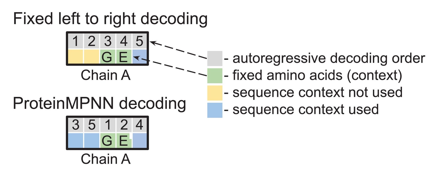
The authors of ProteinMPNN also experimented with random decoding order, where instead of decoding from N terminus to C terminus, a random order was chosen. This could come in handy in situations where the middle of a sequence is known and one wants to design the surrounding sequence elements.
The last trick the authors experimented with was backbone noise. In backbone noise, a little gaussian noise is added to each of the residue backbone coordinates during training. This is useful for situations where the exact atomic resolution of a structure is not known, so we want the model to be robust to small errors in atomic coordinates. Training with backbone noise resulted in a decrease in sequence recovery for the PDB data, where atomic resolution is known, but an increase in accuracy for the AlphaFold test data, where it is not.
Virtual beta carbon positions are an estimate of where the beta carbon should be in the residue based on the position of the backbone atoms and ideal bond angles and bond lengths.
The NH2 end of the polypeptide chain: the one residue in the chain that has a nitrogen not part of a peptide bond to a carbonyl carbon.
The only carboxyl carbon in polypeptide chain that is not part of a peptide bond. It is on the opposite end of the protein sequence from the N terminus.
What percent of residues in the sequence were correctly predicted.