
AlphaFold2 Deep Dive Part 2: The Input Data
All about the three main inputs to AlphaFold2: the query sequence, the MSA, and templates

Protein Inputs
The inputs to the AlphaFold2 model are, no surprise, proteins. For each protein, we take some raw data on that protein, extract features from it, and then run it through the AlphaFold2 model to get our 3D structure prediction. To take a deeper look at the raw data and the process of extracting features, let’s choose an example protein.
Our Example Protein: Myoglobin
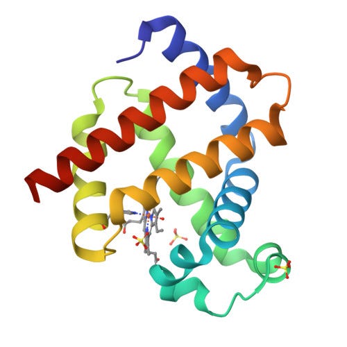
We’ll pick as our example protein human myoglobin, which is a muscle cell protein found used to store and supply oxygen to the muscles. Interestingly enough, myoglobin in other animals (due it’s binding to iron) is what makes meat look red! See the figure above for a diagram of its 3D structure.
We pick myoglobin because it is not too long in sequence length and not too complex in structure. Moreover, it has a well known structure as experimentally determined by scientists. Information on myoglobin is found in the Protein Data Bank (PDB). PDB is a repository containing the 3D atomic coordinates of tens of thousands of proteins (and other biological molecules) that biologists have painstakingly obtained through experimental methods, such as X-ray crystallography. As we mentioned in the last post, x-ray crystallography involves purifying a protein, crystallizing it, shooting x-rays at it then determining the arrangements of the atoms based on the diffraction patterns of the x-rays.
When we go to find human myoglobin in the PDB here, we actually find mutant myoglobin, which means some residues are different from the residues on the true human myoglobin. The reason it is a mutant is that it can often be quite hard to crystallize a protein in order to x-ray it, so modifying the protein slightly is the only way structural biologists can successfully crystallize it. This mutant is described as a K45R, C110A mutant, which means two residues from the original protein were replaced: a lysine at position 45 in the sequence was replaced with an arginine and a cysteine at position 110 was replaced with an alanine.
The Input Data
Now that we have our example protein, we can extract the raw data we need from it.
In AlphaFold2, three pieces of data are used as input for each protein: the protein’s amino acid residue sequence (typically called the query sequence), its multi-sequence alignment, and templates, which are the structures of evolutionary similar proteins.
The Query Sequence
To get our query sequence, the residue sequence of the protein we want to predict a structure for, we either extract it from particular file found on PDB. During training, we get the query sequence from a file called a coordinate file. It’s named as such because it contains the 3D coordinates of every atom in the protein. This is important during training because these coordinates from the experimentally determined structure of the protein, which we use as a ground truth label to help train AlphaFold to do our structure prediction task.
The main coordinate file format is the Macromolecular Crystallographic Information File or mmCIF file format, which you can download from PDB. To obtain the human myoglobin coordinate file, you can find it by manually searching on the PDB website. Here it is!
The coordinate file for myoglobin is quite large with a lot of data on the atomic coordinates and how the structure was measured and a lot of other metadata. For our purposes, however, we just need a veeeery small but critical slice of it, the sequence.
Here is the snippet of the coordinate file dealing with the input residue sequence for our protein in question:
_entity_poly.pdbx_seq_one_letter_code ;GLSDGEWQLVLNVWGKVEADIPGHGQEVLIRLFKGHPETLEKFDRFKHLKSEDEMKASEDLKKHGATVLTALGGILKKKGHHEAEIKPLAQSHATKHKIPVKYLEFISEAIIQVLQSKHPGDFGADAQGAMNKALELFRKDMASNYKELGFQG;Similarly, if we were doing inference, we would extract the FASTA file for human myoglobin from PDB, which just contains sequence info and no coordinate info. It’s a tiny file, so we’ll show it in it’s entirety:
3RGK_1|Chain A|Myoglobin|Homo sapiens (9606) GLSDGEWQLVLNVWGKVEADIPGHGQEVLIRLFKGHPETLEKFDRFKHLKSEDEMKASEDLKKHGATVLTALGGILKKKGHHEAEIKPLAQSHATKHKIPVKYLEFISEAIIQVLQSKHPGDFGADAQGAMNKALELFRKDMASNYKELGFQGIt’t almost identical to the coordinate file sequence snippet, but the first line of metadata differs between the two.
Ok let’s unpack the coordinate file snippet.
First we have the “data item name”: _entity_poly.pdbx_seq_one_letter_code, which is used in cif files as a sort of field name to describe the data and this one basically just means the sequence of amino acid residues in our protein as expressed with the “one-letter code”. The one-letter code uses the letters in the alphabet to represent each amino acid (remember 20 amino acids and 26 letters in the English alphabet 😉).
Below we show the mapping from letter to amino acid residue:
A: alanine
C: cysteine
D: aspartic acid
E: glutamic acid
F: phenylalanine
G: glycine
H: histidine
I: isoleucine
K: lysine
L: leucine
M: methionine
N: asparagine
P: proline
Q: glutamine
R: arginine
S: serine
T: threonine
V: valine
W: tryptophan
Y: tyrosine
The next piece of the snippet is data item value, which is the actual sequence:
GLSDGEWQLVLNVWGKVEADIPGHGQEVLIRLFKGHPETLEKFDRFKHLKSEDEMKASEDLKKHGATVLTALGGILKKKGHHEAEIKPLAQSHATKHKIPVKYLEFISEAIIQVLQSKHPGDFGADAQGAMNKALELFRKDMASNYKELGFQG
As we can see from the number of characters in the sequence, the human myoglobin protein is 153 residues long. It starts with glycine, leucine, serine, aspartic acid, etc.
Also, we see that the 45th residue is R (arginine) and the 110th is A (alanine), which are two residues that make this mutant different from the true human myoglobin protein.
This is the main input to AlphaFold2. That’s it. From there it will predict the 3D structure! Pretty crazy huh? Well, it’s not quite that simple. The inputs to the machine learning model are a lot more complex, but this sequence is the starting point, which is pretty crazy! We’ll dive into how we preprocess this sequence in the next post! Let’s move on to the next raw input, which we derive in part from the sequence: the multi-sequence alignment.
The Multi-Sequence Alignment (MSA)
A multi-sequence alignment (MSA) is a collection of protein sequences arranged in such a way as to show their evolutionary relation. More concretely, it is a text file consisting of one protein sequence on each line encoded using the one-letter code as shown above. The first line is our query sequence and the subsequent lines are protein sequences that share a common evolutionary ancestor with the query protein. Before we go any further on that, let’s dive into the how and why we need an MSA.
Homology and How it Helps Us Figure Out Structure
To describe MSA’s first we have to start with… homology. Two proteins are homologous if they are evolutionarily similar i.e., if they originated from a common ancestor. One way this common ancestry occurs is with orthologs, which are two or more proteins that are the same functional protein, but exist in different organisms. For example, human insulin and ape insulin are orthologs as they have different residue sequences, but have the same function and often a similar structure in their respective organisms. The second type of homolog is paralogs, which are two similar protein sequences which arise when a gene is duplicated, such that the DNA contains two identical copies of the gene. In the paralog case, the duplicated gene doesn’t have the same evolutionary pressure to remain the same and code for the same protein as the original one is already there to fulfill that purpose! As such, the duplicated gene frequently develops mutations and diverges from the original gene. Since genes are recipes for proteins, this can result in a slightly different protein from the original that it “descended” from.
Why is homology important for protein structure prediction? It turns out that finding homologs of our query protein sequence can be quite helpful in our quest to predict its 3D shape. How? One utility is templates, which are the structures of the proteins that are homologs to our query sequence. Basically, if we assume that evolutionarily similar protein sequences have similar structure then knowing the homologs’ structures can give us a big hint into how the protein in question is structured. More on templates in the next section. Templates sound great, buuut as we covered in the previous post, scientists know a lot more protein sequences than they do structures, so in most cases we don’t have the structures of a given protein’s homologs. However, we can still make use of the sequences of these homologs!
It turns out that even with no structural information, the comparison of two sequences with common ancestry can give us hints to their structure. Specifically, covariation information on pairs of residues or simply how two residues change together across multiple homologs can inform us if residues are close to each other in 3D space. Covariation occurs if multiple homologs consistently having a glycine and leucine at positions 5 and 10, for instance, even while the rest of the surrounding residues between 5 and 10 differ across the sequences. Similarly, covariation can occur if whenever a homolog has a different residue than glycine at position 5, the leucine at position 10 consistently changes in that homolog.
Both of these covariation examples likely mean these two residues are in proximity in the final tertiary structure and moreover, that there was an evolutionary pressure to keep them folded that way, which affected how the DNA and the corresponding protein sequences evolved. This simple covariation example is a nice illustration, but often it is more complicated to find true, useful covariation as there is the risk of spurious or transitive correlations1. To avoid these correlations with a veneer of covariation, we need some statistical rigor and thus need to look at how all residues in a protein change across many homologs. Many, many homologs.
Fantastic Homologs and Where to Find Them (and align them)
So where do we find all these homologs?
The answer is protein databases. In protein databases, scientists catalog billions of protein sequences collected from sources like soil samples, analysis of genomes, plants and animal microbiomes, or even culling through scientific literature. Most databases are either organized by individual sequence or by clusters of sequences, which are grouped together based on how similar they are. For example, if a database is clustered with 90% sequence identity that means it groups together sequences that are at least 90% exactly the same (residue by residue). In AlphaFold2, there are four main protein sequence databases that they search to generate MSA’s. There is the MGnify Protein Database, which has 2.4 billion protein sequences clustered to 90% identity (718 million clusters) and the UniRef90 database containing 460 million sequences clustered to 90% identity (184 million clusters). Finally, there is the Uniclust30 database, which clusters proteins from UniProtKB ( a ~250 million proteins database) to clusters of proteins that have about 30% identity, and Big Fantastic Database (BFD), which consists of 65 million clusters of 2.2 billion protein sequences clustered at 30% similarity. The databases clustered to 90% identity really only remove very close duplicates, so they really are more considered sequence databases. The 30% clustered databases, on the other hand, are more organized by protein family than individual sequence, so they have fewer items to search, which can be cheaper to search.
Similarity implies Homology
If we just have database of sequences how can we figure out which ones share a common ancestor with our query protein? Don’t we need some phylogenetic trees or something?
The answers are similarity and no. Usually, if two sequences are similar that implies homology. This is because a pair of sequences being similar just by chance would be very unlikely, so if they’re similar they probably share an ancestor. Indeed, statistical calculations can actually determine how unlikely it would be that they would be similar by coincidence. The reverse: homology implying similarity is not necessarily the case, which means very distant homologs might be very difficult to find. As we will see later, some homology detection algorithms are better than others at finding distant homologs, which is a trait we call sensitivity.
Just finding these similar sequences, however, is not enough to construct our MSA. If we want to accurately track how particular residues co-vary across homologs, especially homologs whose sequences might differ substantially, we need to align the sequences. By align we mean line up the homologous sequences with the “query” sequence such that the aligned residues are homologous. For two residues to be homologous they must both correspond to the same residue in their common ancestor even if the actual residue identity has changed as the protein has evolved. Since each sequence is a line of text and each character is a residue, we can stack the lines on top of the other. Any characters directly on top of each other in the stack will form a vertical column one character wide. This column corresponds to a homologous residue. This stack of sequences is essentially what a multi-sequence alignment (MSA) is, an alignment of protein sequences formulated in such a way as to reveal their evolutionary relation.
To align homologs that contain residues that are not present in all homologs, gaps are often inserted in the string of letters to make sure that each sequence is correctly ordered, but still aligned with the others. One could think of these gaps as representing an evolutionary addition or subtraction of a residue as the sequence evolved. See more in the Anatomy of an MSA section.
MSA Generation Algorithms (Homology Detection and Alignment)
Ok so how do we actually measure similarity and conduct our alignment to create our MSA? It turns out computing an optimal MSA, which means every residue in every sequence is aligned such that each column of the alignment has residues that all descended from the same residue of their common ancestor, is an NP-complete problem. This generally means the only way to guarantee the correct solution is to try every possible way of aligning sequences, which is computationally intractable given how combinatorially immense the solution space is. Because “correct” homolog alignment is not feasible, many algorithms have been invented that use heuristics to come to a suboptimal, but still quite good, solutions in a realistic amount of time. These algorithms vary in their speed and accuracy.
Up until recently the main class of detection and alignment algorithms were sequence-based methods. These methods involve comparing the sequences in the database to the query sequence to figure out how similar they are. If the sequences are determined to be similar enough, they are deemed to be a “hit” and then the algorithm figures out in what order to progressively align each “hit” sequence to the query sequence.
AlphaFold2, on the other hand, makes use of a more sophisticated class of methods called profile-based methods. This class of methods will build a “profile” of the query sequence, which is basically a probability distribution specifying the probability of seeing each of the 20 amino acids at each position in the sequence. The profile is then used to compare sequences in the database by computing how likely each sequence is under the distribution. Profile-based methods are often used as they are more “sensitive” meaning they can find more distantly related homologs, which are homologs whose sequences don’t look very similar, but nonetheless shared a distant ancestor.
The profile-based methods that AlphaFold2 uses build profiles using a probabilistic model called a Hidden Markov Model (HMM). HMM’s are beyond the scope of this post, but essentially they are a type of probabilistic model that is well-suited to model the probability distribution of sequential data. HMM’s consist of modeling the sequence of residues as a sequence of hidden or latent random variables, one for each residue. Each of these latent variables can “emit” one of the 20 possible amino acid residue outcomes as governed by an emission probability distribution. The latent variable outcomes for proteins usually consist of “match”: the residue corresponds to the same residue as the common ancestor, “deletion”: the residue at this position in the common ancestor is missing in this sequence, or “insertion”: an extra residue exists in this sequence that doesn’t correspond to any common ancestor. These latent variables are governed by a transition probability distribution, which models, for example, the probability of the next residue being a match state given the current one is a delete state, etc.
AlphaFold2 utilizes two different HMM profile algorithms for detecting and aligning: JackHMMER and HHBlits. JackHMMER is what is called a profile-sequence method. First, it uses sequence-sequence methods to find a few homologs from the database then it aligns and builds an HMM profile from those initial “hits”. Once it has the initial profile, it follows the general procedure of profile-sequence methods, where each sequence in the database is scored against the profile (calculate how likely the sequence is under the probability distribution) and then the top scoring ones are used to rebuild the profile. The process then repeats with the updated profile. JackHMMER detects and aligns sequences from the MGnify and UniRef90 databases because those are essentially sequence databases (clustered to 90% similarity).
For the cluster databases (Uniclust30 and BFD), AlphaFold uses HHBlits, which is an HMM “profile-profile” method (also known as an HMM-HMM method). Recall that in cluster databases each entry in the database is a cluster or family of multiple sequences. These databases are perfect for profile-profile methods because in these methods, a profile is created from each cluster in the database. In HHBlits these cluster profiles are HMM profiles and each cluster profile is scored against the query HMM profile by checking how closely they agree in how likely a sequence would be under each profile. The sequences from the highest scoring cluster profiles are then are used to update the query profile.
Generating an MSA
Now that we know why we need MSA’s and how they’re built, let’s take a look at one!
Since we have our “query” myoglobin sequence, it’s relatively easy to generate an MSA using free tools easily found online. We use an implementation of HHBlits run on Max Planck Institute servers applied to the UniRef30 database, which they host. UniRef30 uses the sequences from the UniRef90 database described above, but clusters them at 30% similarity, like the UniClust30 database previously described. After running HHBlits on our sequence and downloading the resulting file, we have our MSA. Let’s take a look!
Anatomy of an MSA
Here’s a truncated snippet of our MSA:
#A3M#
>6532126
GLSDGEWQLVLNVWGKVEADIPGHGQEVLIRLFKGHPETLEKFDRFKHLKSEDEMKASEDLKKHGATVLTALGGILKKKGHHEAEIKPLAQSHATKHKIPVKYLEFISEAIIQVLQSKHPGDFGADAQGAMNKALELFRKDMASNYKELGFQG
>UniRef100_A0A151NHW1 Myoglobin n=1 Tax=Alligator mississippiensis TaxID=8496 RepID=A0A151NHW1_ALLMI
QLSDQEWKHVLDIWTKVESKLPEHGHEVIIRLLQEHPETQERFEKFKHMKTADEMKSSEKMKEHGTNVFTALGNILKQKGNHAEVLKPLAKSHALEHKIPVKYLEFISEIIVKVIAEKYPADFGADSQAAMRKALELFRNDMASKYKEFGYQD
>UniRef100_A0A7K9BBU7 Myoglobin (Fragment) n=1 Tax=Dromaius novaehollandiae TaxID=8790 RepID=A0A7K9BBU7_DRONO
LSNSETPGVAGpWLCSRWQLSGLTSPPASVCRLFHDHPETLDRFERFKGLTTPDQMKASEDLKKHGVTVLTQLGKILKLKGKHEAELKPLAQTHATKHKIPVKYLEFISEVIIKVIAEKHSADFGADSQAAMKKALELFRNDMASKYKEFGFQG
>UniRef100_M3YM80 Myoglobin n=1 Tax=Mustela putorius furo TaxID=9669 RepID=M3YM80_MUSPF
GLSDGEWQLVLNVWGKVEADLAGHGQAVLISLCQgleSRKEEKKRDPAHACVSSRRSLFVSQDLLFHSDAFLVSLGH-------------------rsflapvsgengqsqktqpahhAQHHRQPWNTEKFISDAIIQVLQSKHAGDFGAEAQAAMKKALELFRNDIAAKYKELGFQG
>UniRef100_A0A1C4HCU8 Myoglobin (Fragment) n=1 Tax=Protopterus annectens TaxID=7888 RepID=A0A1C4HCU8_PROAN
-ASAAQWDTTLKFWeAHVAGDLKKHGHEALVRLFLKNKDSQKHFPKFKDL-ASeAEMRGSDGLKNHGETVFTALGKALQQRDGIANELRPLAVTHSQNHKIPLEEFENICEVIDVYLAEIC-PDYAGETRTSVKAVLDVFSQSMTTLYGEV---->UniRef100_A0A1C4HCZ4 Myoglobin (Fragment) n=1 Tax=Protopterus annectens TaxID=7888 RepID=A0A1C4HCZ4_PROAN-LSEVQWNELLAFWdKYVAPSSSEHGKHILIRMFQTEKATQTLFSKFKDI-PTSDLAVNADVKKHGGVVVDFLGKLLKLKGQNDSQLHTMAESHKNKHKIPLDYFQVISSVIDVYVNENL-PEEYAPVRQSMKSALNQIANGLKDNYAKV----
Ok this is a lot to look at with a naked, untrained eye, so let’s walk through it.
This is an excerpt from the first 13 lines of an A3M file, which is a standard file format for representing MSA’s. Shown here are six sequences (the query human myoglobin sequence first followed by 5 homolog sequences). The lines that start with “>” describe what the protein is. The first line is described with a numerical id assigned to the query I made (6532126), so that just means human myoglobin for our purposes. The subsequent “>” lines contain the protein name (all of them are myoglobin orthologs in this example). Also, detailed after “tax=” is the genus and species the protein is found in. Let’s remove these metadata lines to make it easier to see the alignment and then we’ll add in parentheses which species (in English not Latin) the myoglobin came from. In addition, we’ll remove one of the lungfish (Protopterus annectens) fragments too. Finally, we’ll just show the first 20 residues and the last 20 residues for each sequence (separated by a space):
GLSDGEWQLVLNVWGKVEAD ALELFRKDMASNYKELGFQG (Human myoglobin) QLSDQEWKHVLDIWTKVESK ALELFRNDMASKYKEFGYQD (American alligator myoglobin)
LSNSETPGVAGpWLCSRWQL ALELFRNDMASKYKEFGFQG (Emu myoglobin)
GLSDGEWQLVLNVWGKVEAD ALELFRNDIAAKYKELGFQG (Ferret myoglobin)
-LSEVQWNELLAFWdKYVAP ALNQIANGLKDNYAKV---- (West African Lungfish myoglobin fragment 2)
Ok that’s better!
MSA’s are usually sorted by e-value, which measures how similar a sequence is to the query sequence. The e-value measurement is a bit confusing: it measures for a given “hit” sequence how many hits on average could one find by chance that have a better alignment score given the size of the database we are searching. I find it a bit confusing to wrap my head around e-value, but basically a lower score means a closer match between a given sequence and the query sequence by similarity and homology. According to our result human myoglobin is actually closest evolutionarily to alligator myoglobin followed by emu and ferret myoglobin. Wow!
If all the homologs are just myoglobin from other organisms, couldn’t we just extract all the myoglobin sequences from a database instead of painstakingly comparing every sequence or profile to our query sequence profile? Not quite. First off, in looking at the entire MSA we generated it doesn’t just have myoglobin sequences, but it does have mostly sequences from the globin family (hemoglobin, neuroglobin, cytoglobin, etc). It does, however, have some uncharacterized proteins and some other non-globin ones, which are had higher e-scores and are more distant homologs. Distant homologs are still quite useful for protein structure prediction to give us more sequences to work with to calculate covariation. Moreover, it seems to me that seeing what conservations and substitutions exist in even the most distant homologs could give us a strong signal on residue contacts.
Ok let’s dig into our truncated MSA.
If a sequence has an upper case letter in the column, that means it’s a match, which means the alignment algorithm has determined that the residue at this position is homologous to the query sequence’s residue at this position. Remember homologous residues are ones that correspond to the same particular residue in their common ancestor. They don’t actually have to be the same residue to be a match. If they are the same residue that is called a conservation. If a match at a certain position is a different residue than that of the query, that is called a substitution. As we can see looking at the first column, the first residue of the ferret myoglobin is a glycine (G) just like the human myoglobin’s first residue, so that’s a conservation. Consequently, the glutamine (Q) and lysine (L) from the alligator and emu are examples of substitutions at that position.
If there is an extra residue in a hit sequence that doesn’t correspond to a homologous residue in the query sequence, that is called an insertion. Insertions are often represented with a lower case letter or not shown at all since it messes up the alignment as it adds an extra character. The twelfth residue in the emu myoglobin sequence is a lower case p, so that is an insertion.
Lastly, a deletion occurs when the homologous residue at this position in the query sequence is missing from the hit sequence at this same position. In deletions, a gap (denoted with a dash: ‘-’) is placed in the column, so the sequences can stay aligned. For example, the West African lungfish myoglobin’s first two residues are a lysine (L) and a serine (S), which match up nicely with the second and third residue of the query sequence. It is, however, missing a homologous residue to the query sequence’s glycine at position one, which is a deletion and that’s why the lungfish sequence starts with a “-”.
Another interesting phenomenon that we observe is the first and fifth residue in the query sequence are glycine (G) and the first and fifth of the alligator myoglobin sequence are glutamine (Q). Residues 1 and 5 seem to change together, which is an example of them co-varying. Of course, we only see them changing together in one hit sequence; we’d have to see a recurring statistically pattern across the MSA to conclude anything. If we did see a co-varying pattern at 1 and 5, however, then it may suggest that these two residues in human myoglobin are related to each other structurally; perhaps they would be near each other in the 3D conformation of the protein. To truly find statistically significant covariation that denotes spatial proximity, we would need to do some complex calculations across all residues in all sequences in the MSA. This sounds like a job for a massive neural network and that is indeed what we will feed this MSA to. In the next post, we’ll show how we preprocess and “featurize” an MSA to prepare it to be input to the AlphaFold2 neural network.
Templates
While MSA rows are sequences of homologs to the query sequence, templates are the structures of homologs to the query sequence. Because proteins evolve a lot slower than their sequence, a sequential homolog to our query sequence likely has a very similar structure to our query protein structure. Why do structures evolve slower than sequences? Well for one, there are multiple different residue combinations that can result in the same shape, so even though the protein sequence mutated there was evolutionary pressure for the protein to keep the same shape. This means that even as the sequence mutated due to random mutations, the genetic mutations that kept the same functional shape were fixed. Hence, structure of homologs can potentially imply query protein structure!
How do we find these templates? We actual do so in an almost identical way to finding homologs for an MSA. Namely, we use an HMM profile-profile detection and alignment algorithm to get the closest homologs. But the catch is we search a database that only contains sequences that we know the structure of. Specifically, AlphaFold uses an algorithm called HHSearch, which is an HMM-HMM detection and alignment algorithm very similar to HHBlits. HHSearch is applied to PDB70, a cluster database of protein sequences from PDB that we know the structure for. To save computation time, AlphaFold2 uses one of the query sequence HMM profiles built during the MSA construction. Specifically, they took the MSA built using JackHMMER with UniRef90 and then converted the MSA to an HMM (relatively straightforward to do) before inputting it to HHSearch.
Extracting a Template
Ok let’s find a protein to use as a template as an example. We’ll use a tool on the Max Planck Institute website called HHPred (super similar to HHSearch) applied to PDB70. We find in our results (also a screenshot below), our top hit is loggerhead sea turtle myoglobin.
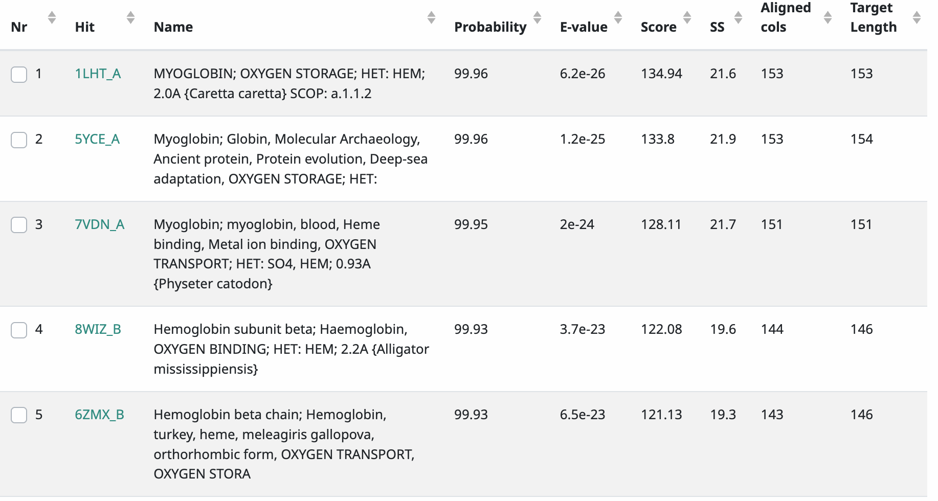
Essentially, this means HHSearch determined that of the proteins with known structures, loggerhead sea turtle myoglobin is the one that is closest in sequence similarity to our query protein. Ok great that’s the protein we’ll use for our template! For templates, we need the protein coordinates, so we’ll download the turtle myoglobin coordinate file on the PDB website just like we did for the human myoglobin when we extracted the query sequence.
The Template Coordinates
Ok so let’s unpack our template coordinate file. What we are interested in for our template is not the sequence, but the coordinates in three-dimensional space of all the (non-hydrogen) atoms in the protein.
These are actual experimentally determined coordinates of the atoms using x-ray crystallography!
So here is a snippet from the turtle myoglobin coordinate file containing the coordinate information for the first 3 residues:
ATOM   1    N  N   . GLY A 1 1   ? 25.690  -3.870  0.688  1.00   49.41 ? 1   GLY A N   1
ATOM   2    C  CA  . GLY A 1 1   ? 26.168  -2.610  1.118  1.00   43.34 ? 1   GLY A CA  1
ATOM   3    C  C   . GLY A 1 1   ? 25.648  -1.599  0.058  1.00   39.15 ? 1   GLY A C   1
ATOM   4    O  O   . GLY A 1 1   ? 25.339  -2.135  -1.003 1.00   38.46 ? 1   GLY A O   1
ATOM   5    N  N   . LEU A 1 2   ? 25.623  -0.293  0.383  1.00   28.11 ? 2   LEU A N   1
ATOM   6    C  CA  . LEU A 1 2   ? 25.166  0.618   -0.622 1.00   22.02 ? 2   LEU A CA  1
ATOM   7    C  C   . LEU A 1 2   ? 26.366  1.330   -1.219 1.00   19.40 ? 2   LEU A C   1
ATOM   8    O  O   . LEU A 1 2   ? 27.360  1.344   -0.527 1.00   20.30 ? 2   LEU A O   1
ATOM   9    C  CB  . LEU A 1 2   ? 24.212  1.742   0.032  1.00   19.17 ? 2   LEU A CB  1
ATOM   10   C  CG  . LEU A 1 2   ? 22.788  1.309   0.228  1.00   15.13 ? 2   LEU A CG  1
ATOM   11   C  CD1 . LEU A 1 2   ? 22.743  0.210   1.246  1.00   19.08 ? 2   LEU A CD1 1
ATOM   12   C  CD2 . LEU A 1 2   ? 22.134  2.474   0.834  1.00   16.76 ? 2   LEU A CD2 1
ATOM   13   N  N   . SER A 1 3   ? 26.213  1.916   -2.377 1.00   16.54 ? 3   SER A N   1
ATOM   14   C  CA  . SER A 1 3   ? 27.326  2.685   -2.938 1.00   19.22 ? 3   SER A CA  1
ATOM   15   C  C   . SER A 1 3   ? 27.286  4.082   -2.314 1.00   21.84 ? 3   SER A C   1
ATOM   16   O  O   . SER A 1 3   ? 26.254  4.455   -1.704 1.00   17.92 ? 3   SER A O   1
ATOM   17   C  CB  . SER A 1 3   ? 27.108  2.858   -4.453 1.00   20.57 ? 3   SER A CB  1
ATOM   18   O  OG  . SER A 1 3   ? 25.806  3.491   -4.678 1.00   34.71 ? 3   SER A OG  1
Ok let’s unpack this snippet. This snippet is in the mmCIF tabular style, where multiple different values are repeated.
This snippet contains information about each “heavy” (non-hydrogen) atom in the first three residues of the protein. Each row is called a record and corresponds to one atom and each column contains data about that atom.
Let’s unpack the sixth row as an example skipping columns with . or ?:
ATOM 6 C CA . LEU A 1 2 ? 25.166 0.618 -0.622 1.00 22.02 ? 2 LEU A CA 1
The first column (ATOM) corresponds to the PDB record type. ATOM means this record contains information about x,y,z coordinates for atoms in the residues of the protein. Contrast with a PDB record type of HETATM, which coordinates for atoms not found in the residues of the protein, like co-factors or ions.
The second column (6) is the atom serial number, which is basically just the index of the atom in the protein. The index is enumerated from the first atom of the first residue of the protein to the last atom of the last residue. If no coordinate information is missing, the serial number is the same as the row number.
The third column is the atom type, which just corresponds to the element of the atom (e.g., C for carbon, N for nitrogen, etc.).
The fourth column is the atom name, such as which carbon is it in the residue (CA for alpha carbon, CB for beta carbon, C for carbonyl carbon, etc.).
The sixth column (LEU) is the 3-letter code for the residue name that the atom is part of (e.g., GLY is glycine, LEU is leucine, and SER is serine).
The seventh column (A) is the chain identifier. Many proteins consist of multiple distinct polypeptide chains, so the letters: A, B, C, etc. denote which chain this atom comes from.
The eighth column (1) is the unique chain identifier. In some proteins, for example, they have multiple polypeptide chains (multimers), but some of them consist of the identical residue sequence (homomers), so this data value just counts chemically distinct chains.
The ninth column (2) is the residue index, indicating the residue’s position in the sequence, so leucine is the second residue of the turtle myoglobin polypeptide.
The most important columns! The 11th, 12th, and 13th columns (-1.513, 18.492, 16.328) are the x, y, and z coordinates of the atom in 3D space and the units are in angstroms (Å)!
So to review this is the 6th atom, which is an alpha carbon on the 2nd residue in the sequence, which is the amino acid leucine. This is the 1st polypeptide chain (A) of the protein and the 1st unique one (1). This atom is found in 3D Cartesian space at [-1.513, 18.492, 16.328] angstroms from the origin.
There we go. There’s the relevant data for a template from a coordinate file. In the next post, we will cover how we preprocess the template coordinates for input to the model!
If residues at position 1 and 2 have contact and so do 2 and 3, then there is correlation between 1 and 3 even if 1 and 3 don’t touch.