
AlphaFold2 Deep Dive Part 3: Embedding the Input Data
Featurizing and embedding our input data into learnable representations!

Note: the code in this post is used for illustrative purposes only and should not be used for any reproducing or reimplementing of AlphaFold2 (see their github repo for that).
Note: Some knowledge of machine learning and Python is necessary to understand this post!
The Input Representations
For the sequence data, as any raw input that we want to process with deep learning, like an image, sentence, or audio file, we have to translate it into a language the model understands: numbers. This translation process is called feature extraction. We extract features from the protein sequence to create the pairwise representation, from the MSA to create the MSA representation and the extra MSA representation and from the templates to create the template representation Let’s go through each representation one by one.
A. The Pairwise Representation
The pairwise representation is an encoding of the pairwise interaction between EVERY possible pair of residues. Why do we want to do this? Well, as part of determining the 3D structure of our myoglobin, we want to know how close in 3D space each residue is from the others. As the AlphaFold2 model trains, it will ideally refine the pairwise representation such that it implicitly encodes the relative distances of the residues. Then, hopefully, we can decode this interaction representations into accurate atomic coordinates!
To create this pairwise representation, we need our human myoglobin residue sequence, which we can get from the coordinate file. In the previous post, we downloaded our mmCIF coordinate file manually. Here we will do it programmatically using some python API’s.
Downloading the coordinate file
We make use of rcsbapi, which is a python toolkit provided by RCSB for querying the PDB and import some key classes and functions:
from rcsbapi.search import TextQuery
from rcsbapi.data import DataQuery
from rcsbapi.search import search_attributes as attrs
Next, we search query the database for the PDB id of our protein in question, human myoglobin.
q1 = TextQuery(”Myoglobin”)
q2 = attrs.rcsb_entity_source_organism.scientific_name == “Homo sapiens”
search_query = q1 & q2
results = search_query()

# We grab the first result because we’re confident the searching will
# return the most relevant one, but we’ll double check.
pdb_id = next(iter(results))
Let’s double check that the result is 3RGK (which we know from actually manually searching) and that 3RGK is actually the PDB id for human myoglobin:
dq = DataQuery(input_type=’entries’, input_ids=[pdb_id], return_data_list=[’struct.title’])
data_q_result = dq.exec()
print(data_q_result[’data’][’entries’][0])
This code should output:
{’rcsb_id’: ‘3RGK’, ‘struct’: {’title’: ‘Crystal Structure of Human Myoglobin Mutant K45R’}}
Ok ‘Crystal Structure of Human Myoglobin Mutant K45R’ that sounds right! Now armed with our PDB id, we can download the coordinate (mmCIF) file! We can use a great python toolkit called biopython to do this!
import Bio
from Bio.PDB import PDBList

# Grab the mmcif file for our PDB id and download it to our current
# working directiory ('.')
PDBList().retrieve_pdb_file(pdb_code=pdb_id, pdir=’.’, file_format=’mmCif’)
Now that we have our file, let’s parse it to get our sequence. We use a nice little class from BioPython called MMCIFParser.
from Bio.PDB import MMCIFParser

pdb_id = ‘3RGK’
parser = MMCIFParser()
structure = parser.get_structure(pdb_id, filename=f”{pdb_id}.cif”)

# Extract sequence one letter code.
seq = parser._mmcif_dict[’_entity_poly.pdbx_seq_one_letter_code’][0].replace(’\n’, ‘’)

num_res = len(seq) # number of chars = number of residues.
Ok let’s check if we extracted the sequence correctly
print(f”Sequence is {num_res} residues long and is: {seq}”)This code should output:
Sequence is 153 residues long and is: GLSDGEWQLVLNVWGKVEADIPGHGQEVLIRLFKGHPETLEKFDRFKHLKSEDEMKASEDLKKHGATVLTALGGILKKKGHHEAEIKPLAQSHATKHKIPVKYLEFISEAIIQVLQSKHPGDFGADAQGAMNKALELFRKDMASNYKELGFQG
There it is! Our myoglobin sequence that we were looking at in the previous post!
Embedding the Query Sequence
The myoglobin residue sequence is all we need to create our first input representation, the pairwise representation. The first step in embedding our sequence is vectorizing it, converting it from a string of characters to a vector of numbers. We vectorize it by transforming each residue letter to a one-hot encoding of the residue. To help us do that let’s first enumerate the “alphabet” of all one-letter codes used for amino acids.
aa_alphabet = [’A’, ‘C’, ‘D’, ‘E’, ‘F’, ‘G’, ‘H’, ‘I’, ‘K’, ‘L’, ‘M’, ‘N’, ‘P’, ‘Q’, ‘R’, ‘S’, ‘T’, ‘V’, ‘W’, ‘Y’]Recall, one-hot encoding is a way of encoding a sequence of discrete symbols, like our residue one-letter codes. Each residue in the sequence is converted to a 20-dimensional vector (because 20 possible amino acids/letters in the one-letter code alphabet) containing all zeros except at the index of that residue’s amino acid code.
For example, the first residue of myoglobin is glycine, which is the 6th letter in the amino acid 1-letter code alphabet. As such, the one-hot encoding of glycine is vector of 20 zeros, except the 6th element is a 1. The next residue, leucine, is 10th in alphabet, so first all zeros, except the 10th is a 1, etc.
Let’s code this up! We’ll use numpy, a very powerful scientific computing library.
import numpy as np

# Make the 153 vectors of 20 elements.
seq_one_hot = np.zeros([num_res, len(aa_alphabet)], np.uint8)

# Figure out where each residue lies in the alpahbet.
inds = [aa_alphabet.index(residue_code) for residue_code in seq]
inds = np.array(inds)

# Set the correct 0 to a 1 for each residue’s vector.
seq_one_hot[np.arange(num_res), inds ] = 1
Let’s check our work here for the first five residues:
print(f”The first five characters of the sequence are: {seq[:5]}”)
print(f”\nThe first five vectors of our one-hot encoding are:”)
print(’ ‘ + ‘ ‘.join(aa_alphabet))

for vec in seq_one_hot[:5]:
    print(vec)
This should help us visualize if our one-hot encoding is correct. Here’s what it should look like:
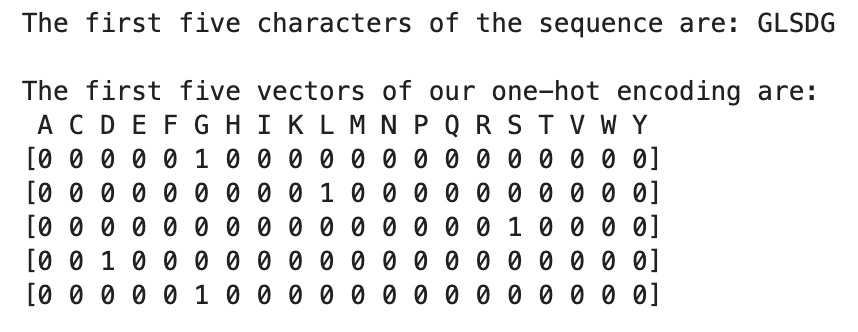
Looks good!
Ok this is the part where a knowledge of machine learning is likely needed. Now that we have transformed our sequence of characters to a set of vectors (actually more of a 2D matrix), we can start doing some learnable deep learning operations on it.
In order to do that, we convert our numpy array to a PyTorch tensor, which will build a computation graph of all the operations we do on the tensor. PyTorch is a popular python deep learning library. By tracking every operation, this graph will allow us compute gradients of our final loss function with respect to the learnable parameters that make up the model (backpropagation) and then we can use those gradients to adjust the learnable parameters (gradient descent).
In AlphaFold2, they project each 20-dim vector to to c_z dimensions TWICE, where c_z in practice is 128.
import torch
from torch import nn

cz = 128
# Convert to torch tensor, so we can do ML
seq_rep = torch.from_numpy(seq_one_hot).float()

num_res, seq_feat_len = seq_rep.shape

lin_a = nn.Linear(seq_feat_len, cz)
lin_b = nn.Linear(seq_feat_len, cz)

# Project twice.
a, b = lin_a(seq_rep), lin_b(seq_rep)
Now if we print out the first 8 dims of the representation for the first five residues, we see that they are no longer vectors of zeros with one 1, but long vectors of random (for now) floats:
for vec in a[:5,:8]:
   print(vec.data)
This should output something that looks like this:

This transformation from one-hot encoding to projection is “learnable” in that over time the machine learning process will adjust how the one-hot encoding is transformed, so that these projections are best suited to encode the sequences such that our final structure prediction task is more accurate!
Encoding Pairwise Interactions
Now let’s get to the pairwise part of pairwise representation.
We want to encode the interaction between all possible pairs of residues and every vector represents one residue. Moreover, order is considered in this case, so residue 1 with residue 6 is a different interaction than residue 6 with residue 1. Since human myoglobin is 153 residues long, we need to construct 153^2 interaction representations. We will represent each interaction as a vector, so we really are computing a size 153 x 153 tensor, where each element is a vector. We encode the interaction by just adding every vector from the first projection of our residues, a, with every vector b, resulting in the final 153 x 153 x 128 tensor, which we’ll refer to in code as z.
Essentially, we want the ijth position of this tensor to be formed by adding the ith residue’s first projection, a[i,:], with the jth residue’s second projection, b[j,:]. Similarly, the jith position of this tensor would be formed by adding the jth residue’s first projection, a[j,:], with the ith’s second, b[i,:].
Instead of doing a nested for loop like so, which would be slow:
z = torch.zeros((num_res, num_res, cz))
for i in range(num_res):
    for j in range(num_res):
        z[i,j] = a[i,:] + b[j,:]
We can do this with just one line of code taking advantage of PyTorch’s broadcasting and vectorizing ability:
# Add every residue representation in a with every one in b.
z = a[:, None, :] + b[None, :, :]
When we add None in the indexing of a tensor it adds a dummy dimension of size 1 to the tensor, so a[:, None, :] is of shape 153,1,128 and b[None, :, :] is of shape 1,153,128. When you do an elementwise operation, like addition, between two tensors, each dimension of the tensor must match the corresponding dimension of the other tensor unless one of the dimensions of is of size 1. In that case, the tensor with dimension of 1 is conceptually replicated to match the size of the larger dimension in the other tensor before executing the elementwise operation. This way we can efficiently do elementwise operations without using a lot of unnecessary memory or writing a slow Python for loop. See these resources on broadcasting and vectorizing for more information.
Relative Position Encoding
Above, we added each pair of residue projections, which encoded the interaction between each pair of residues, but in the encoding there is no notion of how close they are together in the primary sequence. For example, z[4,11], encodes the interaction between the 4th and 11th residues, but nowhere in the encoding is the notion that they are 7 positions away from each other in the primary sequence.
To remedy this we add to the representation the relative position of the two residues (how many residues are between them). This is similar to positional encoding in transformers!
First, we enumerate each residue from 0 to 152 and then (using broadcasting) subtract every residue’s index from every other residue’s index. This gives us how many residues between any given residue pair. A positive valued relative positions means the the first residue in the pair is later in the sequence than second and vice versa for negative values. Lastly, we clip these distances to be between -32 and 32 as anything more than 32 residues away is considered quite far away and doesn’t need it’s own encoding. Here’s some code:
# Enumerate every residue.
res_ind = torch.arange(num_res)

# Use broadcasting to subtract each pair of indices.
rel_pos = res_ind[:, None] - res_ind[None, :]

# Max out the relative position at 32.
rel_pos = torch.clip(rel_pos, min=-32, max=32)
Let’s check our work! The distance between our 2nd residue leucine and our 7th residue tryptohan should be -5 and between our 6th glutamic acid and our 3rd serine should be 3.
# Indexing from 0, so 1,6 instead of 2,7, etc.
print(rel_pos[1, 6])
print(rel_pos[5, 2])
This should output:
tensor(-5)tensor(3)
Looks right!
These relative positions are one-hot encoded then linearly projected to c_z and then added to our pairwise representation tensor, `z`
# Create the bins for one-hot encoding
v_bin = torch.arange(-32,33)
We can do the one-hot encoding in one line by1:
1. Comparing every relative position to all 65 bins to check for equality by broadcasting the `==` operator resulting in a tensor, where for each residue pair there is boolean vector that is true at the index of the correct bin and false for the others.
2. We then just convert this True, False vector to 1’s and 0’s using int() and voila one-hot encoding!
# Compare each relative position to all 65 bins -> boolean array
# Convert the boolean array to 1's and 0's.
# The result is equivalent to one-hot encoding.
rel_pos_1hot = (rel_pos[:, :, None] == v_bin[None, :]).int()
Now we just projecte the relative position to the same dimension as the pairwise representation and add it to the pairwise representation to get our final pairwise representation:
lin2 = nn.Linear(rel_pos_1hot.shape[-1], cz)
proj_rel_pos = lin2(rel_pos_1hot.float())
z += proj_rel_pos
That’s it. That’s the pairwise representation: adding the embeddings of each pair of residues and then adding the relative positions. Let’s look at the MSA representation!
B. The MSA Representation
Clustering and cropping the MSA
The MSA file we described in the previous post was actually quite long. Although, we only showed five hit sequences, the file actually had over 1,000 hits (🙀)! Actually, the AlphaFold2 authors configured HHBlits to have no limit in the number of output sequences. Furthermore, the limit of hit sequences they set when searching the two different sequence databases with jackHMMER tool was 5,000 and 10,000. All this to say: there are a lot of sequences in the MSA’s generated for AlphaFold2. Trying to process all multi-thousands of these sequences in AF2 could be quite expensive computationally.
In fact, to process the MSA representation, AlphaFold2 --spoiler alert-- uses self-attention; the same self-attention used in the transformers that we find in today’s LLM’s. Unfortunately, the computational and memory cost of self-attention in transformers scales quadratically with respect to the number of sequences, but only linearly with respect to the feature size of each sequence. In the MSA case, there are actually separate self-attention operations for MSA’s over the columns (self-attention across residues in the same hit sequence) and the rows (self-attention across residues at the same position in every sequence). As such, limiting the number of rows AND columns we use in the MSA would go a long way in reducing the computational load. Reducing the feature dimension of a given residue embedding, on the other hand, is not as important. AlphaFold2 takes advantage of this insight in their preprocessing of the raw MSA in three ways: block deletion, residue cropping, and msa clustering.
Block Deletion
First, to eliminate the number of rows, they do block deletion, which involves randomly removing a few blocks of consecutive sequences in the MSA. This works because MSA’s are usually ordered by how close of a match they are to the query sequence2. Hence, deleting contiguous blocks of an MSA can reduce sequences that are very similar anyway and don’t provide much signal, while increasing diversity by including sequences of differing similarity to the query (varying levels of how close the common ancestor of the query sequence is).
Residue Cropping
Second, to reduce the number of columns, they employ residue cropping, where they randomly crop a contiguous 256-residue long region (same region for every hit sequence of course) to use for training (during fine-tuning they expand it to 384). Human myoglobin is only 153 residues long, so no need to do residue cropping in this example.
MSA Clustering
Third, and most crucially, the authors randomly choose a subset of hit sequences to use for training (128 during training and 512 during fine-tuning). Because the feature dimension isn’t as crucial for reducing computation and memory cost, they add statistics computed from the unused MSA sequences as extra features for the hit sequences they do use.
Let’s dive into the code for the embedding of MSA’s using clustering. We won’t show block deletion (done before clustering and embedding) for brevity (😜) nor residue cropping (done after clustering and embedding) as it is not necessary for this short of a protein sequence.
Embedding the MSA in Code
Here, we will just use the MSA file we generated in the previous post, which we’ll call hhblits_full.a3m. First, let’s just read in the raw text from the file:
with open(’hhblits_full.a3m’, ‘r’) as f:
    lines = f.readlines()
Next, we will remove the annotation lines starting with “>” that just describe the protein and also remove insertions (represented as lower case letters), which we remember are “extra” amino acids in the “hit” protein that don’t align well with the query protein.
# Remove metadata lines and strip new line \n
raw_msa = [line.strip(’\n’) for line in lines if not line.startswith(’>’) and not line.startswith(’#’)]

# Remove lower case letters because those are insertions and they add an # extra unalligned character.
raw_msa = [’‘.join([c for c in line if not c.islower()]) for line in raw_msa]
MSA Clustering
Now, let’s get to clustering. For clustering, we randomly sample 127 MSA sequences and then the 128th is the first row of the MSA, our myolgobin query sequence. Each of these chosen sequences is called a “cluster center”.
import numpy as np
import random
num_clust_tr = 128
num_msas = len(raw_msa)

# The first cluster is always the first seq in MSA because that’s the
# query sequence, so we
# sample from all the rest and then add the 0th in.
cluster_inds = random.sample(list(range(1, num_msas)), k=num_clust_tr - 1)
cluster_inds = [0] + cluster_inds
cluster_msas = np.asarray([raw_msa[i] for i in cluster_inds])
One-Hot Encoding the MSA Cluster Centers
Embedding the MSA is a very similar process to how the input sequence is embedded into the pairwise representation. First, each of the 153 residues in every row of the MSA is one-hot encoded, so we now go from a sequence of 153 characters to a (153, 23) tensor. It’s 23 because 20 amino acids + 1 unknown (’U’) + 1 gap (’-’) + 1 mask token3.
To compute the MSA one hot encoding efficiently, we use some tricks: broadcasting, pre-allocation, and integer array indexing.
alphabet = np.char.array([’A’, ‘C’, ‘D’, ‘E’, ‘F’, ‘G’, ‘H’, ‘I’, ‘K’, ‘L’, ‘M’, ‘N’, ‘P’, ‘Q’, ‘R’, ‘S’, ‘T’, ‘V’, ‘W’, ‘Y’, ‘U’,# unknown            ‘-’, ‘$’])

seq_len = len(raw_msa[0]) # 153

# Convert cluster_msas to char array.
cluster_msas_char = cluster_msas.view(’U1’).reshape(cluster_msas.shape[0], seq_len)
# “U1” means unicode string contraining just one character.
# Broadcast the == operator to determine index of each residue char in
# the alphabet.
residue_ind = np.argmax(cluster_msas_char[:,:, None] == alphabet[None, :], axis=-1)

# Preallocate one-hot msa rep.
msa_1hot = np.zeros((cluster_msas.shape[0], seq_len, len(alphabet)), dtype=np.int64)

# Set the correct element of each residue’s vector of 0’s to 1 using
# integer array indexing.
msa_1hot[np.arange(msa_1hot.shape[0])[:, None],    np.arange(msa_1hot.shape[1]), residue_ind] = 1
MSA Deletion Features
Concatenated to these 23 dimensions are 3 dimensions denoting any deletions to the left of the residue. Remember, a deletion occurs when sequence is missing the homologous residue to the one in the query sequence. For deletions in the MSA the gap character ‘-’ is placed.
cluster_has_deletion: 1 if the residue to the left of the given has a deletion, 0 otherwisecluster_deletion_value: The total number of deletions to the left of the given residue squashed to a float between 0 and 1.cluster_deletion_mean: The average number of deletions to the left of a given residue position averaged over all sequences in the MSA.
# We add a feature for if there is a deletion to the left
# boolean array for if residue is a deletion
is_deletion = np.int64(cluster_msas_char == ‘-’)

# Shift to right to indicate whether residue to left is deletion.
cluster_has_deletion = np.roll(is_deletion, 1, axis=1)
cluster_has_deletion[:, 0] = 0 # Set the leftmost feature to 0 as there

# can’t be any res to the left of it.
# Compute total number of deletions to the left by computing a
# cumulative sum using np.cumsum.
deletion_to_left_count = np.cumsum(cluster_has_deletion, axis=1)

# AlphaFold2 squashes the counts to be between 0,1 using the formula
# 2/pi * arctan(d/3), where d is the count.
cluster_deletion_value = (2. / np.pi) * np.arctan(deletion_to_left_count / 3.)
# cluster_deletion_mean counts what the average number of deletions to
# the left of a residue is across all sequences in the cluster.

cluster_deletion_mean_raw = np.repeat(deletion_to_left_count.mean(axis=0, keepdims=True),
repeats=deletion_to_left_count.shape[0], axis=0)

# Squashed to be between 0 and 1
cluster_deletion_mean = (2. / np.pi) * np.arctan(cluster_deletion_mean_raw / 3.)
MSA Profile Features
The last MSA feature is the “MSA Profile” feature. Remember, for each unused MSA sequence we determine which cluster center the sequence is closest to and then consider that sequence a “member” of the chosen cluster. The statistics of each cluster are added as extra features to each cluster center. That way we use fewer sequences, but each sequence (even the unused ones) still contributes somewhat to the prediction. Some of the unused sequences also get used as a separate input (see Extra MSAs). Remember that each row in the MSA is supposed to be a representative sequence for a cluster of unused sequences, so another 23 dimensions are concatenated that capture the cluster’s probability distribution of amino acid types at this residue position.
# Separate out the MSA’s not chosen as cluster centers.
extra_msas = np.asarray([raw_msa[i] for i in range(num_msas) if i not in cluster_inds])

# Convert extra_msa tensor to a char array to easily compare to
# cluster_msas_char.
extra_msas_char = extra_msas.view(’U1’).reshape(extra_msas.shape[0], seq_len)

# Compute hamming distance between each extra msa and every cluster
# center msa.

hamming_distances = np.sum(extra_msas_char[:, None] != cluster_msas_char[None, :], axis=-1) # More broadcasting!


# Assign to each extra msa a cluster id of whichever cluster center is  # the closest in hamming distance.
extra_msa_cluster_ids = hamming_distances.argmin(axis=1)

# One hot encode extra msa.
extra_residue_ind = np.argmax(extra_msas_char[:,:, None] == alphabet[None, :], axis=-1)

extra_msa_1hot = np.zeros((extra_msas.shape[0], seq_len, len(alphabet)), dtype=np.int64) # Preallocate.

extra_msa_1hot[np.arange(extra_msa_1hot.shape[0])[:, None], np.arange(extra_msa_1hot.shape[1]), extra_residue_ind] = 1 # Integer indexing.

# For each cluster id, sum 1-hot encodings of members and divide by
# number of members to get profile.
# Done with python for loop to make more readable. Vectorizing this
# doesn’t really result in much a speedup in practice.
msa_profile = np.zeros((num_clust_tr, seq_len, len(alphabet)), dtype=np.float64)
for i in np.unique(extra_msa_cluster_ids):
    # Sum one-hot to get counts for each residue for the given cluster.
    seqs_in_cluster_i = extra_msa_1hot[extra_msa_cluster_ids == i]
    cluster_i_profile = seqs_in_cluster_i.sum(axis=0)
    # Divide counts by total members to get profile statistics.
    cluster_i_profile = np.divide(cluster_i_profile, seqs_in_cluster_i.shape[0], where=seqs_in_cluster_i.shape[0]!= 0)
    msa_profile[i] = cluster_i_profile
Concatenating All the Features Together
Now we just concatenate all the features to form the MSA representation
msa_feat = np.concat(
    (msa_1hot,
     cluster_has_deletion[:, :, None],
     cluster_deletion_value[:, :, None],
     cluster_deletion_mean[:, :, None],
     msa_profile),
    axis=-1)
print(msa_feat.shape)
(128, 153, 49)
Embedding the Features
Now that we created our MSA features we can embed them into vector representations. First, we convert our numpy arrays to torch tensors, so we can compute gradients during training. Embedding the features consists of linearly projecting the MSA features then adding a projection of the query sequence to each and every MSA row feature.
import torch
from torch import nn

c_m = 256

# Convert to torch tensor, so we can include projections in
# computational graph.
msa_rep = torch.from_numpy(msa_feat).float()

# Linearly project the MSA representation to c_m dimensions.
lin1 = nn.Linear(msa_rep.shape[-1], c_m)
msa_rep = lin1(msa_rep)

# Convert to torch tensor.
query_seq_1hot = msa_1hot[0]
query_seq = torch.from_numpy(query_seq_1hot).float()

# Project the 1-hot query sequence to c_m dimensions as well.
lin2 = nn.Linear(query_seq.shape[-1], c_m)
query_seq_proj = lin2(query_seq)

# Add the query sequence peojection to each and every msa row
# projection.
final_msa_rep = query_seq_proj[None, :, :] + msa_rep # Broadcasting
C. The Extra MSA Representation
The extra MSA’s are the subset of the MSA sequences that were not selected as cluster centers. They featurized in a very similar way to the MSA cluster centers: one-hot encoding each residue in each sequence (23 dims) plus two dimensions denoting deletion information (2), but this time no features related to cluster statistics. Similar to the MSA, each 25-dim residue feature is projected to c_e dimensions, which in this case 64.
We already one-hot encoded the extra MSA’s above, so we just need to add in the deletion features and project to 64 dims.
# Compute deletion features.
extra_is_deletion = np.int64(extra_msas_char == ‘-’)
extra_has_deletion = np.roll(extra_is_deletion, 1, axis=1)
extra_has_deletion[:, 0] = 0
extra_deletion_to_left_count = np.cumsum(extra_has_deletion, axis=1)
extra_deletion_value = (2. / np.pi) * np.arctan(extra_deletion_to_left_count / 3.)

# We just concatenate the deletion info to get the extra msa features.
extra_msa_feat = np.concat((extra_msa_1hot, extra_has_deletion[:,:, None], extra_deletion_value[:,:, None]),  axis=-1)

# Project the features to 64 dims.
c_e = 64
lin_extra = nn.Linear(extra_msa_feat.shape[-1], c_e)
extra_msa = lin_extra(torch.from_numpy(extra_msa_feat).float())
D. The Template Representation
As we covered in the previous post, templates are the 3D structures of proteins that are homologous to our query protein. Moreover, as we know, the raw input of templates are the 3D coordinates of all the non-hydrogen atoms in the homolog protein as catalogued in a coordinate file. These 3D coordinates will then be featurized into “template pair features” and then added to the pairwise representation. The motivation here is to embed/encode some structural priors into the input.
First let’s download our template’s coordinate file.
from Bio.PDB import MMCIFParser, PDBList
from Bio.PDB.MMCIF2Dict import MMCIF2Dict
import os

pdb_id = ‘1LHT’ # PDB id of seaturtle myoglobin.

# Download 1LHT mmcif file
pdbl = PDBList()
filepath = pdbl.retrieve_pdb_file(pdb_code=pdb_id, pdir=’.’, file_format=’mmCif’)

# Create dict of coord file to make it easier to extract coordinates.
cif_dict = MMCIF2Dict(filepath)
Ok so now that we have our template file, we can featurize the coordinates into two main features: template angle features and template pair features.
Template Angle Features
We won’t go too deeply into these since AlphaFold3 ended up scrapping these in their template preprocessing. Basically, the template angle features contain residue torsion angle information. For each residue, there are 3 backbone torsion angles and 4 side chain torsion angles. In the template angle features, each of these angles is parametrized by the sin and cos components of the angles (so 14 total dimensions for each residue). In addition, there is a tensor for the alternative 4 torsion angles for side chains with rotation symmetry (8 dims) and mask tensor indicating if the torsion angle is present in the template (7 dims). Concatenated to these three tensors is the one-hot encoding of the residue type (22 dims) resulting in total a 51-dimensional tensor for each residue in each template. This tensor is processed by a 1-layer MLP and then concatenated to the MSA representation.
Template Pair Features
The template pair features is a size (num_templ, num_res, num_res, 88) tensor. If you notice it has a size (num_res, num_res) inner dimension similar to the pairwise representation. Just like the pairwise representation, it is constructed to capture 88 pairwise features between each possible pair of residues in the sequence. This 88-dimension tensor is composed of the template sequence features, template distogram features, the template unit vector features, and template masks. Let’s cover them each in sequence.
1. Template Sequence Features (44 dims)
Part of capturing the pairwise interaction between two residues in the template is just encoding the the residue identity of the two residues. So this first portion of the template features doesn’t even use the coordinates (just the sequence of the template). The first 44 dimensions of the feature are just the 22-dimensional one-hot encoding of the ith residue (20 amino acids + unknown and gap) concatenated to the one-hot encoding of jth residue.
# Extract the sequence from the coordinate file.
seq = cif_dict[’_entity_poly.pdbx_seq_one_letter_code’][0]
seq = seq.replace(’\n’, ‘’)
num_res = len(seq)
alphabet = [’A’, ‘C’, ‘D’, ‘E’, ‘F’, ‘G’, ‘H’, ‘I’, ‘K’, ‘L’, ‘M’, ‘N’, ‘P’, ‘Q’, ‘R’, ‘S’, ‘T’, ‘V’, ‘W’, ‘Y’,
‘?’, #unknown,
‘-’ # gap
]

# Preallocate one-hot enc tensor.
# Each row is the one-hot encoding of one residue.
seq_one_hot = np.zeros([num_res, len(alphabet)], np.uint8)

# Get index of where to place each 1 in the one-hot encoding.
inds = [alphabet.index(residue_code) for residue_code in seq]
inds = np.array(inds)

# Set the 0 to 1’s where appropriate using integer indexing.
seq_one_hot[np.arange(num_res), inds ] = 1
Next we make a pairwise tensor, where the ijth element is the ith residue’s one-hot encoding concatenated to the jth element’s one-hot encoding. We can do this by using broadcasting to tile rows and columns. So now when we concatenate the two, we get our desired pairwise one-hot encoding.
depth = len(alphabet)
# Tile the tensor to make it a 3D tensor of num_res 2D tensors.
# The kth 2D slice has num_res identical rows, where each row is the
# one-hot encoding of the kth residue.
repeating_rows = np.tile(seq_one_hot[:, None, :], (1, num_res, 1))

# 3D tensor of num_res identical 2D slices, where each 2D slice is seq_one_hot, the original 2D array where each row is a different
# residue’s one-hot encoding.
repeating_arrays = np.tile(seq_one_hot[None, :, :], (num_res, 1, 1))

# Concatenate the two so the “feature” dimension (i, j, :) is the
# concatenation of the ith and jth residue’s one-hot encoding.
templ_seq = np.concatenate((repeating_rows, repeating_arrays), axis=2)
2. Template Distogram Features (39 dims)
The template distogram features encode the distance between every pair of residues. To create template distogram features:
Extract the coordinates (in angstroms) from the coordinate file for each residue’s beta carbon (except for the glycine residue, which doesn’t have a side chain, so no beta carbon, so we use its alpha carbon).
Compute the distance between every beta carbon with every other beta carbon resulting in a $N_{res} \times N_{res}$ tensor, where the $ij$th element is the distance between the ith residue beta carbon and the jth residue’s one.
Discretize each distance by creating 38 bins between 3.25Å and 50.75Å and a 39th for any distance larger than 50.75 and one-hot encoding which bin each distance falls into.
We now will have the template distogram features, a size (num_res, num_res, 39) tensor for each template.
Let’s dive into some code
First to make our job easier, we convert our mmcif file dictionary to a Pandas Dataframe, where the rows are atoms and the columns are the data about each atom.
import pandas as pd
cif_keys = [
            # PDB group type (ATOM for atoms in the residues).
            ’_atom_site.group_PDB’,
            # index of residue (1 is first residue, 2 is second, etc.)
            ‘_atom_site.label_seq_id’,
             # which chain (A, B, etc.)
            ‘_atom_site.label_asym_id’,
             # which atom (just the element e.g. C, N, O)
            ‘_atom_site.type_symbol’,
            # type of atom (CA: alpha carbon, CB: beta carbon, C is
            # carbonyl carbon, N is nitrogen)
            ‘_atom_site.label_atom_id’,
            ‘_atom_site.label_comp_id’, # residue name (e.g. VAL, GLY)
            ‘_atom_site.Cartn_x’, # x coord
            ‘_atom_site.Cartn_y’, # y coord
            ‘_atom_site.Cartn_z’] # z coord

# More readable key names for columns of the dataframe
key_nicknames = [’atom_group’,
                 ‘res_ind’,
                 ‘chain_id’,
                 ‘element’,
                 ‘atom_type’,
                 ‘res_name’,
                 ‘x’,
                 ‘y’,
                 ‘z’]

# Make a dataframe for these keys and values from the mmcif file.
coord_data = zip(*[cif_dict[k] for k in cif_keys])
cif_df = pd.DataFrame(coord_data, columns=key_nicknames)
We also make a dataframe for any atoms that no coordinate info is available for.
missing_coord_info_keys = [
    ‘_pdbx_unobs_or_zero_occ_atoms.label_comp_id’,
    ‘_pdbx_unobs_or_zero_occ_atoms.label_seq_id’,
    ‘_pdbx_unobs_or_zero_occ_atoms.label_atom_id’
    ]

missing_coord_info_nicknames = [’res_name’, ‘res_ind’, ‘atom_type’]
missing_data = zip(*[cif_dict[k] for k in missing_coord_info_keys])
mis_df = pd.DataFrame(missing_data, columns=missing_coord_info_nicknames)
1. Extract the coordinates for the beta carbons
# We filter for actual residue atoms. ATOM means atoms that are actually part of the polypeptide.
res_atom_only_df = cif_df[cif_df[’atom_group’] == ‘ATOM’]

# We just grab the A chain (myoglobin only has an A chain).
res_a_chain_df = res_atom_only_df[res_atom_only_df[’chain_id’] == ‘A’]
true_res_ind = res_a_chain_df[’res_ind’].astype(’int’) - 1 # subtract 1 so we are indexing from 0.
true_res_ind = true_res_ind.rename(’true_res_ind’)
res_a_chain_df = pd.concat([res_a_chain_df, true_res_ind],axis=1).sort_index()

# Do the same for missing residues
true_res_ind = mis_df[’res_ind’].astype(’int’) - 1 # subtract 1 so we are indexing from 0.
true_res_ind = true_res_ind.rename(’true_res_ind’)
mis_df = pd.concat([mis_df, true_res_ind],axis=1).sort_index()
# Extract all rows that are glycine alpha carbons.
gly_ca_df = res_a_chain_df[(res_a_chain_df['res_name'] == 'GLY') & (res_a_chain_df['atom_type'] == 'CA')]
# Extract all non-glycine beta carbon rows.
cb_no_gly_df = res_a_chain_df[~(res_a_chain_df['res_name'] == 'GLY') & (res_a_chain_df['atom_type'] == 'CB')]# Extract any glycine alpha carbons that are missing coordinate info.
mis_gly_ca_df = mis_df[(mis_df['res_name'] == 'GLY') & (mis_df['atom_type'] == 'CA')]
# Extract any non-glycine beta carbons that are missing coordinate info.
mis_cb_no_gly_df = mis_df[~(mis_df['res_name'] == 'GLY') & (mis_df['atom_type'] == 'CB')]
# Combine to have all missing atoms.
all_missing_beta = pd.concat([mis_gly_ca_df, mis_cb_no_gly_df]).sort_values(by=['true_res_ind'])# Concatenate the existing coordinates with the missing ones and sort
# them so the residues are in the original order of the sequence.
cb_or_gly_ca_df = pd.concat([cb_no_gly_df, gly_ca_df, all_missing_beta]).sort_values(by=['true_res_ind'])# Double check all residues are accounted for.
print(len(cb_or_gly_ca_df.true_res_ind.unique()))153
# Extract the x, y, z coordinates.
coords_arr = cb_or_gly_ca_df[['x', 'y', 'z']].astype('float').to_numpy()

# Missing coords will be nan, so conver nans to zeros.
coords_arr = np.nan_to_num(coords_arr, nan=0.0)
2. Compute the distance between residues’ beta carbons.
# Use broadcasting to get the squared diff between every possible pair.
coords_squared_diff = (coords_arr[:, None, :] - coords_arr[None, :, :])**2

# Sum and square to get L2 distance.
coords_dist = np.sqrt(np.sum(coords_squared_diff, axis=-1))
3. Bin each distance
# 38 bins from 3.25 to 50.75
bins = np.linspace(start=3.25, stop=50.75, num=38)

# Add one more bin for any distance greater than 50.75
bins = np.concatenate((bins, np.asarray([50.7501])))

# The bin each distance belongs to is the one it is closest to when you subtract the diatance from every bin.
bin_id = np.argmin(np.abs(coords_dist[:,:,None] - bins[None, :]), axis=-1)

# One-hot encode the distances.
template_dist = np.zeros((num_res, num_res, bins.shape[0]))
template_dist[np.arange(num_res)[:, None], np.arange(num_res)[None, :], bin_id] = 1
3. Template Unit Vector Features (3 dims)
While the distogram features just encode a scalar distance between the residues, the template unit vector features aim to capture exactly where each pair of residues in the template protein are relative to each other. This is achieved by computing for each pair, the vector that points from one residue’s alpha carbon to the other’s. It’s a little tricky to do this, so let’s dive into the code.
A. Defining the local frame (computing 3 unit vectors)
We want each vector to be defined in a local frame, which essentially is a unique coordinate system defined for each individual residue.
To compute our local frames, we need the coordinates of the carbonyl carbon and nitrogen along with the alpha carbon, so let’s extract those.
# Extract alpha carbon (CA), carbonyl carbon (C), and nitrogen (N) 3D coordinates.
ca_df = res_a_chain_df[res_a_chain_df['atom_type'] == 'CA']
c_df = res_a_chain_df[res_a_chain_df['atom_type'] == 'C']
n_df = res_a_chain_df[res_a_chain_df['atom_type'] == 'N']

ca_coords, c_coords, n_coords = (
                        ca_df[['x','y','z']].astype('float').to_numpy(),
                        c_df[['x','y','z']].astype('float').to_numpy(),
                        n_df[['x','y','z']].astype('float').to_numpy(),
)
Now that we have all the coordinates, we can build our local frame. Remember for each distance between the ith and jth residue, we define the frame around the ith residue. All we need to compute each residue’s local frame are 3 unit vectors. These unit vectors must adhere to the following specifications:
the origin must be defined at the global position of the residue’s alpha carbon.
one unit vector,
e1, must point from the alpha carbon to the carbonyl carbon.one unit vector,
e2, must be orthogonal toe1AND in the 2D plane formed by the alpha carbon, carbonyl carbon, and nitrogen.the last unit vector,
e3must be orthogonal .
Compute e1
# vector pointing from alpha carbon to carbonyl carbon
v1 = c_coords - ca_coords

# Make v1 a unit vector by dividing by the norm of itself (sqrt(v1_x^2 + # v1_y^2 + v1_z^2)))
e1 = v1 / np.linalg.norm(v1, axis=-1, keepdims=True)
Compute e2
Remember:
e2should be orthogonal toe1The vector pointing from the alpha carbon to the nitrogen needs to be in the 2d plane formed by the
e1ande2
# Compute vector pointing from alpha carbon to nitrogen.
v2 = n_coords - ca_coords

# Compute the magnitude of the component of v2 that points in the e1 direction using dot prodict b/w e1 and v2.
v2_m1 = np.vecdot(e1, v2)

# Subtract that magnitude pointing in the e1 direction from v2 to get a vector orthogonal to e1.
u2 = v2 - v2_m1[:, None] * e1

# Normalize u2 to get a unit vector
e2 = u2 / np.linalg.norm(u2, axis=-1, keepdims=True)
Compute e3
For e3 there is only one criterion: it must be orthogoanl to both e1 and e2. We can achieve that using a cross product:
e3 = np.linalg.cross(e1,e2)Let’s check that e1, e2, e3 are actually orthogonal. The dot products should all be 0!
assert np.allclose(np.zeros_like(v2_m1), np.vecdot(e1,e2))
assert np.allclose(np.zeros_like(v2_m1), np.vecdot(e1,e3))
assert np.allclose(np.zeros_like(v2_m1), np.vecdot(e2,e3))
Whew!
Now that we have define a local frame for each residue: e1, e2, e3, we can compute the unit vectors between every pair of residues that are within the local frame of the first residue of the frame. First we just compute the vector pointing from every residue to every other residue in the global frame.
B. Compute pairwise distances in the global coordinate frame.
# Vector pointing from every residue alpha carbon to every other one in # the global coordinate frame.
ca_dist = ca_coords[:, None, :] - ca_coords[None, :,  :] # broadcasting
C. Express pairwise distances in terms of residue-specific local frame.
# Computing the e1,e2, and e3-components of each xyz vector.
# Dot product between each pairwise distance vector and it's corresponding local frame unit vectors.
templ_dist_vector = np.stack((np.vecdot(ca_dist, e1), np.vecdot(ca_dist, e2), np.vecdot(ca_dist, e3)), axis=-1)

# Normalize the vector to get a unit vector.
templ_dist_vector_norm = np.linalg.norm(templ_dist_vector, axis=-1, keepdims=True)
templ_unit_vector = np.divide(templ_dist_vector, templ_dist_vector_norm, out=templ_dist_vector, where=templ_dist_vector_norm != 0.0) #  If the magnitude of the vector is 0, then keep the unnormalized vector.
Voila! Our template unit vector features!
Template Masks (2 dims)
The last two dims are two masks, `template_pseudo_beta_mask` and `template_backbone_frame_mask`, which indicate whether the beta carbon coordinates (or alpha carbon for glycine) and the backbone atom coordinates (alpha carbon, carbonyl carbon, and nitrogen) are present in the coordinate file respectively. For each pair of residues the mask for each is multiplied and then concatenated to the representation.
Compute template_pseudo_beta_mask
# Preallocate the beta_mask to all ones.
beta_mask = np.ones((num_res, 1), dtype=int)

# Grab the index of missing atoms from the all_missing_atoms dataframe
# and set those to 0.
beta_mask[all_missing_beta['true_res_ind'].astype('int').to_numpy()] = 0

# The template_pseudo_beta_mask is only one if both pairs of residues
# have beta carbon coordinates.
templ_pseudo_beta_mask = beta_mask[:, None] * beta_mask[None, :]
Compute template_backbone_frame_mask
# Get any missing ca, c, or n.
mis_ca_df = mis_df[mis_df['atom_type'] == 'CA']
mis_c_df = mis_df[mis_df['atom_type'] == 'C']
mis_n_df = mis_df[mis_df['atom_type'] == 'N']

# Preallocate masks for the backbone atoms to one.
ca_mask, c_mask, n_mask = np.ones((num_res, 1), dtype=int), np.ones((num_res, 1), dtype=int), np.ones((num_res, 1), dtype=int)

# Set each mask to 0 for the residues that have coordinates missing.
ca_mask[mis_ca_df['true_res_ind'].astype('int').to_numpy()] = 0
c_mask[mis_c_df['true_res_ind'].astype('int').to_numpy()] = 0
n_mask[mis_n_df['true_res_ind'].astype('int').to_numpy()] = 0

# Are all three backbone atoms present?
backbone_mask = ca_mask * c_mask * n_mask

# templ_backbone_frame_mask is only 1 if both residues in the pair have # coordinates.
templ_backbone_frame_mask = backbone_mask[:, None] * backbone_mask[None, :] # broadcasting.
Template Pair Features: Putting it All Together
Ok now we just concatenate all the template features to get one big template tensor. Let’s double check the shape is right.
# Concatenate all the template features to get the full num_res x
# num_res x 88 tensor!
template_pair_feat = np.concatenate((templ_seq, template_dist, templ_unit_vector, templ_pseudo_beta_mask, templ_backbone_frame_mask), axis=-1)

print(template_pair_feat.shape)
(153, 153, 88)
Great! Now we project it to 64 dimensions with a learned linear layer.
ct = 64

# Convert to torch because the linear projection is part of the learned model.
template_pair_feat = torch.from_numpy(template_pair_feat).float()

# Project!
lin1 = nn.Linear(template_pair_feat.shape[-1], ct)
templ_repr = lin1(template_pair_feat)

print(templ_repr.shape)
torch.Size([153, 153, 64])
There we have it! The features for our 3 main inputs (plus an extra feature set for extra MSA). Check out the next post to learn about how we transform these features using the Evoformer, the meat of the AlphaFold2 model!
The AF2 algorithm instead does this by subtracting the relative position from every bin in v_bin, taking ther absolute value, then finding the argmin and using that as the index, then making an array of all zeros and setting the zero at that index to 1. This accomplishes the same thing!
Technically, the metric used is “e-value”, a measure of given the size of the database, how unlikely would it be that this sequence is only similar to query sequence by pure coincidence and not some evolutionary relationship. I don’t find this metric to be the most intuitive way of thinking about it, but alas.